


Blog · FP&A Insights
Beyond "8% behind budget": variance analysis that explains, not just reports
A headline variance is arithmetic, not analysis. Here is how to decompose revenue and cost variances properly, with the formulas, a worked example, and how the AI engine in Seizmic FP&A makes it a monthly habit.
By Hardus Odendaal, Subject Matter Expert, Seizmic · 1 November 2026
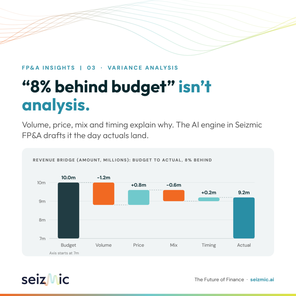
A number is not an explanation
Every month, in finance teams around the world, a version of the same sentence goes into the board pack: "Revenue is 8% behind budget."
It is accurate. It is also almost useless. It tells the executive team that something moved, but not why it moved, whether it will happen again, or who should do something about it. It is arithmetic, not analysis.
Variance analysis is one of the oldest disciplines in management accounting, and one of the most underused. Most finance teams know the theory of volume, price and mix. Far fewer apply it consistently every month, because the data needed to do it properly is spread across systems and the time needed to stitch it together is not there.
In this article I want to go deeper than a LinkedIn post allows. I'll walk through how a revenue variance should be decomposed, with the formulas and a worked example. I'll cover the cost side that matters most in manufacturing, material and labor. I'll look at the pitfalls that make variance analysis misleading, what good commentary looks like, and how the AI engine in Seizmic FP&A turns this from a quarterly luxury into a monthly habit.
Why headline variances fail the Office of the CFO
A headline variance compresses several different business stories into one number. Two companies can both be 8% behind budget for completely different reasons:
1. One sold fewer units because a key customer delayed a program launch. That is a volume problem, and the response is commercial: pipeline, customer engagement and capacity planning.
2. The other sold the planned volume, but more of it went to lower-margin products and customers. That is a mix problem, and revenue may even look fine while gross margin quietly erodes.
The headline number treats these as the same thing. The board conversation, the accountable owner and the corrective action are completely different.
There are three further problems with stopping at the headline:
It hides offsetting movements. A favorable price variance can mask an unfavorable volume variance. The net looks small, so nobody asks the question, until the price increase runs its course and the volume problem is still there.
It confuses timing with performance. Revenue that landed a month early or late is not the same as revenue that was won or lost. Treating them the same leads to over-reaction one month and complacency the next.
It gives no owner. "Revenue is down" belongs to everyone, which means it belongs to no one. "Volume is down at two customers" belongs to the account managers. "Price realization slipped on the new product range" belongs to commercial. Decomposition creates accountability.
For the Office of the CFO, the purpose of variance analysis is not to explain the past. It is to direct attention: to tell the leadership team which levers moved, by how much, and which of those movements will repeat if nobody acts.
The revenue bridge: volume, price, mix and timing
A revenue bridge walks from budget to actual in a sequence of steps, each isolating one driver. The standard decomposition uses four.
Volume is the effect of selling more or fewer units in total, valued at the budgeted average price. It answers: if everything else had gone to plan, what would the change in units alone have done to revenue?
Volume = (actual total units − budget total units) × budget average price
Budget average price = budget revenue ÷ budget units
Mix is the effect of selling a different combination of products or customers than planned. Each line is compared with what it would have sold if the actual total had been split in the budgeted proportions, and the difference is valued at that line's budget price.
Mix = Σ (actual units of the line − actual total units × budget mix % of the line) × budget price of the line
Mix is positive when the business sells more of its higher-priced lines than planned, and negative when it sells more of the lower-priced ones.
Price is the effect of selling at a different rate than planned, measured on the units actually sold.
Price = Σ actual units of the line × (actual price − budget price)
Timing captures revenue that is real but landed in a different period than budgeted: a shipment pulled forward, a milestone invoice billed early, or an order that slipped into next month. Timing is not a formula so much as a classification. It matters because it reverses: a favorable timing variance this month is usually an unfavorable one next month.
Together, volume, mix and price reconcile exactly to the total revenue variance on unit-based sales. Timing sits alongside them for revenue that is not driven by units in the period. The order matters, and I come back to it in the pitfalls below.
A worked example
Take a manufacturer with two product lines: a premium assembly (Product A) and a standard component (Product B). All amounts are in US dollars.
Line
Budget units
Budget price
Budget revenue
Actual units
Actual price
Actual revenue
Product A
30,000
$200.00
$6,000,000
21,400
$220.00
$4,708,000
Product B
50,000
$80.00
$4,000,000
49,000
$87.60
$4,292,400
Total
80,000
$125.00 avg
$10,000,000
70,400
$9,000,400
In the same month, a tooling recovery invoice of $200,000 that was budgeted for next month was billed early. Reported revenue is therefore $9,200,400 against a budget of $10,000,000: the familiar "8% behind budget".
Now decompose it:
1. Volume: 70,400 units were sold against 80,000 budgeted, a shortfall of 9,600 units. Valued at the budget average price of $125, that is a volume variance of −$1,200,000.
2. Mix: at the budget split (37.5% A, 62.5% B), 70,400 units would have been 26,400 of A and 44,000 of B. The business actually sold 5,000 fewer of A and 5,000 more of B. Valued at budget prices, that is −$1,000,000 on A and +$400,000 on B, a mix variance of −$600,000.
3. Price: Product A sold $20 above budget on 21,400 units (+$428,000) and Product B sold $7.60 above budget on 49,000 units (+$372,400), a price variance of +$800,400.
4. Timing: the early tooling invoice adds +$200,000, which will reverse next month.
Step
Amount
Running total
Budget
$10,000,000
Volume
−$1,200,000
$8,800,000
Price
+$800,400
$9,600,400
Mix
−$600,000
$9,000,400
Timing
+$200,000
$9,200,400
Actual
$9,200,400
The headline said "8% behind". The bridge says something far more useful:
The real problem is volume, concentrated in the premium product. That is a commercial conversation about Product A customers.
The price increase landed and is working, but it is covering for the volume gap. Without it, the business would be 16% behind.
The mix shift towards Product B is costing revenue and, almost certainly, margin, because premium assemblies usually carry a higher contribution per unit.
Part of the month's result is borrowed from next month. The true underlying gap is closer to 10% than 8%.
That is four distinct messages, three owners and one warning, from a number that originally said only "down".
The cost side in manufacturing: material and labor
In manufacturing, revenue is only half the story. Material and labor are typically the two largest cost drivers in cost of sales, and they need the same decomposition. Here the comparison is against standard cost for the output actually produced, not against the static budget, so that volume does not contaminate the efficiency picture.
Material splits into price and usage.
Material price = (actual price − standard price) × actual quantity used
Material usage = (actual quantity used − standard quantity for actual output) × standard price
A price variance belongs to procurement: supplier increases, exchange rates, freight, spot buys. A usage variance belongs to operations: scrap, yield, rework, engineering changes or bills of material that no longer reflect how the product is built.
Labor splits into rate and efficiency.
Labor rate = (actual rate per hour − standard rate per hour) × actual hours
Labor efficiency = (actual hours − standard hours for actual output) × standard rate per hour
A quick example. A plant has a standard of 2 labor hours per unit at a standard rate of $30 per hour. It produces 10,000 units, so the standard allows 20,000 hours, or $600,000. It actually works 21,500 hours at an average of $31.50 per hour, a total of $677,250.
Breaking down the $77,250 overspend:
Rate variance: ($31.50 − $30.00) × 21,500 = $32,250 unfavorable. Overtime premiums and shift allowances pushed the average rate up.
Efficiency variance: (21,500 − 20,000) × $30.00 = $45,000 unfavorable. The plant used 1,500 more hours than the output justified.
The two parts lead to very different conversations. The rate variance is a question for HR and plant leadership about overtime policy. The efficiency variance is a question for operations about downtime, changeovers, training or line balancing. And the two are often linked: a plant running behind on efficiency tends to buy back the lost hours with overtime, which shows up again as rate.
Common pitfalls
Variance analysis done badly can be worse than none, because it gives false confidence. These are the mistakes I see most often.
1. Inconsistent calculation order. Volume, mix and price interact. Calculating price on budget units instead of actual units, or valuing volume at actual prices, moves amounts between buckets. Pick one convention, document it, and apply it every month.
2. Mix defined at the wrong level. Mix only means something at the level where prices genuinely differ: product family, customer, channel or region. Across hundreds of SKUs with similar prices it becomes noise; at total company level it disappears entirely.
3. Comparing costs to the static budget. If the plant produced 15% more than planned, material and labor will be over budget, and that is a good thing. Measure cost variances against a flexed budget so that volume is separated from efficiency.
4. Treating timing as performance. Timing variances reverse. If they are not tagged as timing, the business celebrates a good month and then panics about a bad one, when nothing really changed.
5. Standards that are out of date. Usage and efficiency variances are only as good as the bills of material and labor routings behind them. Out-of-date standards measure the age of the standard, not the performance of the plant.
6. No materiality threshold. Explaining every line creates a long pack that nobody reads. Set thresholds by amount and percentage, and focus commentary on the items that cross them.
7. Analysis without an owner. A variance that is explained but not assigned to someone who can act on it has not finished its job.
From analysis to commentary
The bridge is the analysis. The commentary is what the executive team actually reads. Good variance commentary answers four questions in order:
1. What moved? The driver and the amount, in business language.
2. Why? The underlying cause, as specifically as the data allows.
3. Will it repeat? Permanent, timing, or one-off.
4. What are we doing about it? The action, and who owns it.
Compare two versions of the same commentary for the worked example above.
Typical: "Revenue was 8% below budget due to lower sales, partly offset by price increases."
Useful: "Revenue was $800,000 (8%) below budget. Volume was $1.2m short, almost entirely on Product A, where two customers delayed orders; account managers expect partial recovery in the 9+3. Price increases delivered $0.8m as planned. A shift in mix towards Product B cost $0.6m in revenue and is diluting gross margin. $0.2m relates to a tooling invoice billed a month early and will reverse next month. Underlying performance is therefore 10% behind budget."
The second version is longer, but it takes less time to act on. It tells the leadership team where to look, what is temporary, and what is not.
Writing commentary like this every month, for every material line, is exactly where most finance teams run out of time. It is also exactly where AI can help most.
How the AI engine in Seizmic FP&A does this
The reason most teams stop at the headline is not a lack of skill. It is that the inputs live in different places. The GL holds the amounts. The ERP holds units, prices and bills of material. Customer and product hierarchies often live in spreadsheets maintained by one person. By the time an analyst has pulled it together and reconciled it, the month is closed and the moment to act has passed.
Seizmic FP&A solves the data problem first, and then puts AI on top of it.
One governed model. Seizmic FP&A brings GL actuals, budget, every forecast version, volumes and customer and product data into a single model on the Microsoft Data & AI Platform, with one chart of accounts mapped consistently across entities. Measures such as revenue, gross margin and units are defined once, so the bridge reconciles to the same numbers as the Income Statement in the board pack.
Variance decomposition as soon as actuals land. When the month's actuals load, the AI engine in Seizmic FP&A breaks revenue variances into volume, price and mix by product, customer or region, against the budget or any forecast version. There is no spreadsheet to rebuild and no reconciliation to redo.
Cost next to the volume that drove it. On the cost side, Seizmic FP&A compares live material cost per stock code with the cost in the plan, flags items in the sales plan that have no cost behind them, and puts labor cost by cost center and GL next to the volume actually produced. The Manufacturing Cost Statement and Administrative Cost Statement are generated directly from the same model.
First-draft commentary in business language. The AI engine drafts variance commentary that follows the structure above: what moved, why, whether it will repeat. The analyst reviews it, corrects it where the data cannot know the story (a customer conversation, a plant breakdown), and adds the action and the owner.
Questions in plain language. A CFO or financial controller can ask "which customers drove the volume shortfall on Product A?" or "how much of this month's margin decline is mix?" and get an answer drawn from the governed model, not a guess.
The effect is a change of rhythm. Variance analysis that used to happen at quarter end, if at all, becomes a monthly habit. And the finance team's time moves from building the bridge to deciding what to do about it.
Where to start
If your monthly pack still leads with headline variances, here is a practical sequence to move beyond them.
1. Agree the method. Document how volume, price and mix are calculated, in which order, and at which level. Get the CFO and commercial leadership to sign it off, so the numbers are trusted before they are debated.
2. Get units into the same model as amounts. Most of the effort in variance analysis is joining GL amounts to ERP volumes. Until that join is automated, decomposition will always be a manual, end-of-quarter exercise.
3. Refresh your standards. Review material bills and labor routings for your top products, so usage and efficiency variances measure performance, not out-of-date assumptions.
4. Flex the budget for costs. Compare material and labor to standard cost for actual output, and report the volume effect separately.
5. Tag timing. Make timing an explicit category in the bridge, with a note on when it reverses.
6. Set materiality thresholds. Comment on what crosses them, and nothing else.
7. Standardize the commentary. What moved, why, will it repeat, what are we doing about it, and who owns it. Every time.
8. Let AI do the first draft. Once the data is governed and the method is agreed, the decomposition and the first draft of the commentary can be automated, leaving the team to review, add context and drive action.
Explain, then act
"8% behind budget" will always have a place on the first page of the pack. It just cannot be the whole page.
The value of variance analysis lies in the decomposition: volume, price, mix and timing on the revenue line, and price, usage, rate and efficiency on the cost side. That is what turns a number into a set of decisions, each with an owner.
For most finance teams, the method has never been the barrier. The data and the time have. With the inputs in one governed model and the AI engine in Seizmic FP&A doing the first pass, explaining the month stops being the job, and deciding what to do about it becomes the job.
See variance analysis in Seizmic FP&A
See how Seizmic FP&A turns monthly variances into decisions, on your own numbers.
About the author
Hardus Odendaal is Group CEO of TrueNorth Group, the Data and AI consultancy behind Seizmic, and has worked in data and analytics for finance teams for over 25 years. He works with CFOs and finance leaders in South Africa and the United States on the Microsoft Data & AI Platform and AI-driven FP&A.